Making a network
For this class most of the types of network you will want to make can be produced by metaknowledge. The first three co-citation network, citation network and co-author network are specialized versions of the last three one-mode network, two-mode network and multi-mode network.
First we need to import metaknowledge and because we will be dealing with graphs the graphs package networkx as should be imported
[1]:
import metaknowledge as mk
import networkx as nx
And so we can visualize the graphs
[2]:
import matplotlib.pyplot as plt
%matplotlib inline
import metaknowledge.contour.plotting as mkv
Before we start we should also get a RecordCollection to work with.
[3]:
RC = mk.RecordCollection('../savedrecs.txt')
Now lets look at the different types of graph.
Making a co-citation network
To make a basic co-citation network of Records use networkCoCitation().
[4]:
CoCitation = RC.networkCoCitation()
print(mk.graphStats(CoCitation, makeString = True)) #makestring by default is True so it is not strictly necessary to include
The graph has 601 nodes, 19492 edges, 0 isolates, 4 self loops, a density of 0.108109 and a transitivity of 0.691662
graphStats() is a function to extract some of the statists of a graph and make them into a nice string.
CoCitation is now a networkx graph of the co-citation network, with the hashes of the Citations as nodes and the full citations stored as an attributes. Lets look at one node
[5]:
CoCitation.nodes(data = True)[0]
[5]:
(5308678917494226943,
 {'count': 1, 'info': 'CAVALLERI G, 1974, LETT NUOVO CIMENTO, V12, P626'})
and an edge
[6]:
CoCitation.edges(data = True)[0]
[6]:
(5308678917494226943, 7204849785423671553, {'weight': 1})
All the graphs metaknowledge use are networkx graphs, a few functions to trim them are implemented in metaknowledge, here is the example section, but many useful functions are implemented by it. Read the documentation here for more information.
The networkCoCitation() function has many options for filtering and determining the nodes. The default is to use the Citations themselves. If you wanted to make a network of co-citations of journals you would have to make the node type 'journal' and remove the non-journals.
[7]:
coCiteJournals = RC.networkCoCitation(nodeType = 'journal', dropNonJournals = True)
print(mk.graphStats(coCiteJournals))
The graph has 89 nodes, 1383 edges, 0 isolates, 40 self loops, a density of 0.353166 and a transitivity of 0.640306
Lets take a look at the graph after a quick spring layout
[8]:
nx.draw_spring(coCiteJournals)
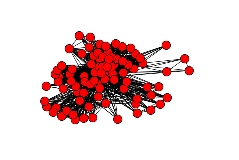
A bit basic but gives a general idea. If you want to make a much better looking and more informative visualization you could try gephi or visone. Exporting to them is covered below in Exporting graphs.
Making a citation network
The networkCitation() method is nearly identical to networkCoCitation() in its parameters. It has one additional keyword argument directed that controls if it produces a directed network. Read Making a co-citation network to learn more about networkCitation().
One small example is still worth providing. If you want to make a network of the citations of years by other years and have the letter 'A' in them then you would write:
[9]:
citationsA = RC.networkCitation(nodeType = 'year', keyWords = ['A'])
print(mk.graphStats(citationsA))
The graph has 18 nodes, 24 edges, 0 isolates, 1 self loops, a density of 0.0784314 and a transitivity of 0.0344828
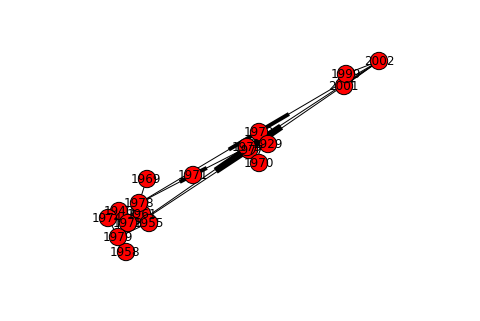
[10]:
nx.draw_spring(citationsA, with_labels = True)
Making a co-author network
The networkCoAuthor() function produces the co-authorship network of the RecordCollection as is used as shown
[11]:
coAuths = RC.networkCoAuthor()
print(mk.graphStats(coAuths))
The graph has 45 nodes, 46 edges, 9 isolates, 0 self loops, a density of 0.0464646 and a transitivity of 0.822581
Making a one-mode network
In addition to the specialized network generators metaknowledge lets you make a one-mode co-occurence network of any of the WOS tags, with the oneModeNetwork() function. For examples the WOS subject tag 'WC' can be examined.
[12]:
wcCoOccurs = RC.oneModeNetwork('WC')
print(mk.graphStats(wcCoOccurs))
The graph has 9 nodes, 3 edges, 3 isolates, 0 self loops, a density of 0.0833333 and a transitivity of 0
[13]:
nx.draw_spring(wcCoOccurs, with_labels = True)
Making a two-mode network
If you wish to study the relationships between 2 tags you can use the twoModeNetwork() function which creates a two mode network showing the connections between the tags. For example to look at the connections between titles('TI') and subjects ('WC')
[14]:
ti_wc = RC.twoModeNetwork('WC', 'title')
print(mk.graphStats(ti_wc))
The graph has 40 nodes, 35 edges, 0 isolates, 0 self loops, a density of 0.0448718 and a transitivity of 0
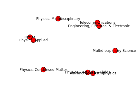
The network is directed by default with the first tag going to the second.
[15]:
mkv.quickVisual(ti_wc, showLabel = False) #default is False as there are usually lots of labels
quickVisual() makes a graph with the different types of nodes coloured differently and a couple other small visual tweaks from networkx’s draw_spring.
Making a multi-mode network
For any number of tags the nModeNetwork() function will do the same thing as the oneModeNetwork() but with any number of tags and it will keep track of their types. So to look at the co-occurence of titles 'TI', WOS number 'UT' and authors 'AU'.
[16]:
tags = ['TI', 'UT', 'AU']
multiModeNet = RC.nModeNetwork(tags)
mk.graphStats(multiModeNet)
[16]:
'The graph has 108 nodes, 163 edges, 0 isolates, 0 self loops, a density of 0.0282105 and a transitivity of 0.443946'
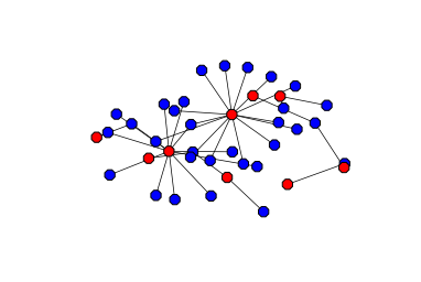
[17]:
mkv.quickVisual(multiModeNet)
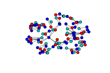
Beware this can very easily produce hairballs
[18]:
tags = mk.tagsAndNames #All the tags, twice
sillyMultiModeNet = RC.nModeNetwork(tags)
mk.graphStats(sillyMultiModeNet)
[18]:
'The graph has 1184 nodes, 59573 edges, 0 isolates, 1184 self loops, a density of 0.0850635 and a transitivity of 0.492152'
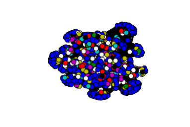
[19]:
mkv.quickVisual(sillyMultiModeNet)
Post processing graphs
If you wish to apply a well known algorithm or process to a graph networkx is a good place to look as they do a good job at implementing them.
One of the features it lacks though is pruning of graphs, metaknowledge has these capabilities. To remove edges outside of some weight range, use dropEdges(). For example if you wish to remove the self loops, edges with weight less than 2 and weight higher than 10 from coCiteJournals.
[20]:
minWeight = 3
maxWeight = 10
proccessedCoCiteJournals = mk.dropEedges(coCiteJournals, minWeight, maxWeight, dropSelfLoops = True)
mk.graphStats(proccessedCoCiteJournals)
[20]:
'The graph has 89 nodes, 466 edges, 1 isolates, 0 self loops, a density of 0.118999 and a transitivity of 0.213403'
Then to remove all the isolates, i.e. nodes with degree less than 1, use dropNodesByDegree()
[21]:
proccessedCoCiteJournals = mk.dropNodesByDegree(proccessedCoCiteJournals, 1)
mk.graphStats(proccessedCoCiteJournals)
[21]:
'The graph has 88 nodes, 466 edges, 0 isolates, 0 self loops, a density of 0.121735 and a transitivity of 0.213403'
Now before the processing the graph can be seen here. After the processing it looks like
[22]:
nx.draw_spring(proccessedCoCiteJournals)
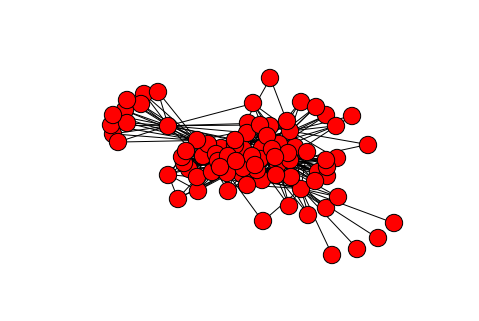
Hm, it looks a bit thinner. Using a visualizer will make the difference a bit more noticeable.
Exporting graphs
Now you have a graph the last step is to write it to disk. networkx has a few ways of doing this, but they tend to be slow. metaknowledge can write an edge list and node attribute file that contain all the information of the graph. The function to do this is called writeGraph(). You give it the start of the file name and it makes two labeled files containing the graph.
[23]:
mk.writeGraph(proccessedCoCiteJournals, "FinalJournalCoCites")
These files are simple CSVs an can be read easily by most systems. If you want to read them back into Python the readGraph() function will do that.
[24]:
 FinalJournalCoCites = mk.readGraph("FinalJournalCoCites_edgeList.csv", "FinalJournalCoCites_nodeAttributes.csv")
mk.graphStats(FinalJournalCoCites)
[24]:
'The graph has 88 nodes, 466 edges, 0 isolates, 0 self loops, a density of 0.121735 and a transitivity of 0.213403'
This is full example workflow for metaknowledge, the package is flexible and you hopefully will be able to customize it to do what you want (I assume you do not want the Records staring with ‘A’).